Overdriving approximation

A physicist, economist, or electrical engineer might object to our story so far:

Good models are made with real math, not formal logic. Nobody uses that stuff, so nobody cares if it doesn’t work. And nobody expects a model to be exact, so this whole “no absolute truth” business is irrelevant. What matters is getting a good enough approximation.

There’s two parts to this, and they are both somewhat true. First, formal logic is indeed mostly useless in practice, for all the many reasons discussed in this Part of The Eggplant.¹ Second, approximate numerical models are powerfully useful in some fields.

However, approximation is not an adequate general understanding for how rational models can work well in the face of nebulosity.

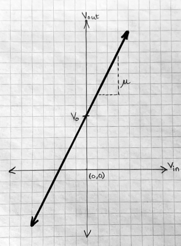
In physics, and many branches of engineering, most models are numerical. Consider an amplifier. The simplest model is linear:

V_out = μ × V_in + V₀

The output voltage is equal to the input voltage times a constant amplification amount μ, plus a constant offset V₀, which is the output for a zero input.

Graphed, this is a straight line:

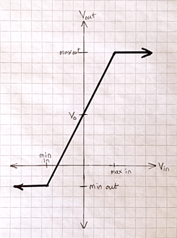
The model is not absolutely true. For small enough positive or negative inputs, it’s very nearly true. However, the amplifier has a limited output range, so large enough inputs can no longer be amplified. You have to limit inputs if you want the amplifier to behave properly. A second, more complex model:

If you measure the output of a vacuum tube guitar amplifier as a function of input, it looks something like this:

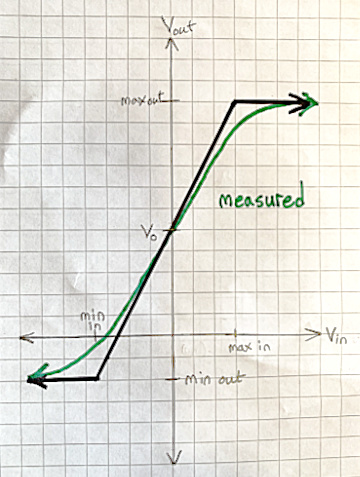
The second model is pretty accurate except near the limits, where the measured behavior is smoothly curved, not sharply kinked. But even the middle section of the curve is never a perfectly straight line. That’s a good approximation, and we can find a numerical bound on how bad it might be—how far it gets from the measured behavior. Successively more complex amplifier models fit the S-shaped curve increasingly accurately—meaning with smaller errors—by taking into account increasingly many physical effects that affect it.

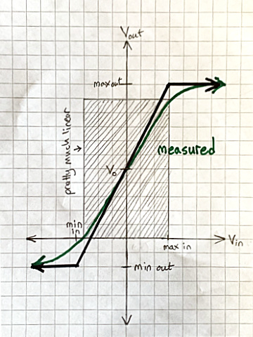
In most amplifier applications, linear behavior is optimal, so you make sure the input voltage stays within the nearly-straight part of the curve:

Vacuum tube guitar amplifiers are an exception. Typically they have deliberately wide non-linear (curved) regions, and are designed so that normal inputs overdrive the amplifier into the curves. That distorts the output—wonderfully, if you like electric blues or hard rock! Increasing overdrive makes the amplified guitar sound successively “warm,” “growly,” and “dirty”; and eventually produces random noise unrelated to what you’re playing on the instrument. Sufficiently high voltage inputs will start to melt components, resulting in short or open circuits; and then internal arcing; and the output will diverge from the model without bound.

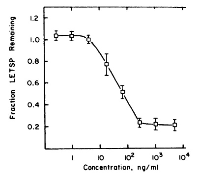
Drugs and poisons often behave analogously to amplifiers. They show a “dose-response relationship”: for example, the more painkillers you take, the less pain you feel. The dose-response relationship is often nearly linear within limits. However, there may be a minimal, threshold dose required to get any effect, and exceeding some maximum dose does not increase the effect. Here’s the dose-response curve for a measured carcinogen effect:

Let’s generalize a pattern from these examples. A numerically approximate model has:

• A domain of applicability, within which it works well.²
• Bounded error, a numerical measure of how wrong it might be if applied within its domain. The error bound may be fixed, or else can be calculated from readily-available parameters.

In earlier chapters, we’ve seen that most knowledge is only sort-of true. The objection at the beginning of this one suggested that sort-of-true knowlege can be understood as an approximation to reality. When its error bound is small enough to get a particular job done, the model is useful, even though it is not absolutely true. If it’s not, you need to find a more accurate model.

This is great when you can get it! An approximate model often works for engineered devices, because they are designed and manufactured to conform to that very model. It is feasible to build computers only because we can—after billions of dollars and decades of research and development effort—manufacture transistors that reliably conform to specifications, within bounded error.

But most sort-of truths aren’t like that. We don’t have numerically approximate models for most things, and aren’t likely to get them. Formal logic is not adequate as a universal framework for constructing rational models, but neither are physics-like numerical formulae. Such models are rare in molecular biology, for example; and when they are possible, they work only “usually.” Unenumerable, mostly unknown factors within a cell may cause a model to break down.

Earlier I used “gene” as an example of a vague term. Some particular bit of DNA is not approximately a gene. It may definitely be one, or not, and it may be “sort of” a gene, but never a gene “to within an error bound.” Likewise, in software engineering, “more-or-less an MVC architecture” is not quantifiable.

To work well, for most rational models, many conditions must hold. I’ll call these usualness conditions.³ Typically, we don’t know what they all are, and there’s no practical way to find out. Some are unknown unknowns. As a consequence, domains of applicability are nebulous, with indefinite boundaries that depend on contexts and purposes.⁴

Truth in physics and physics-like engineering is different from truth in logic, as the objection at the beginning of the chapter noted. Physics is approximately true, not absolutely true (except possibly at the elementary particle scale). But truth elsewhere is different again; it’s usually-true-in-the-sense-adequate-to-get-the-job-done. Ways of reasoning that work for numerically approximate truth do not work for usually-adequate truth, so approximation is not an adequate general model of model adequacy.⁵

We can still do science and engineering in many fields in which error bounds are unavailable. We can still construct good-enough models. A good explanation of rationality has to provide a better understanding of model adequacy than approximation does.

The objection suggested a simple model of model adequacy, the approximation model of models. According to this meta-model, rational models are approximately true, within a well-defined domain of applicability. The approximation model itself has a domain of applicability: it works well for physics-like models. If you try to push it too hard, you overdrive the meta-model into distortion. Applied to software engineering, for example, it can only produce random noise.

An oft-repeated adage, by George Box: “All models are wrong, but some are useful.”⁶ This is usually true, but also sometimes worse than useless. It can be abused as a facile dismissal of the very point it makes, by implying that of course everyone knows there are no absolute truths, and that this isn’t a problem, so we can ignore it. (As the objection suggested.)

But it is a problem: to use a model usefully, you have to find out how and when and why it is useful, and how and when and why it fails. Otherwise, it is likely to burn you at an awkward time, like an amplifier overdriven to the point that it catches fire.

As Box put it: “The scientist must be alert to what is importantly wrong. It is inappropriate to be concerned about mice when there are tigers abroad.”

Inquiry into how and when and why a model works is central to meta-rationality.